Executive Summary and Impact
Regional energy forecasting is fundamentally a system-boundary problem. By disaggregating 1.37 lakh consumer connections into distinct sectoral processes and separating organic growth from inorganic shocks (such as industrial parks and EV plazas), we build an architectural system model rather than relying on naive time-series extrapolation.
Core Thesis
Infrastructure demand is not a single time series waiting to be extrapolated. It is the aggregate behavior of a physical system, and forecasting it requires understanding what that system contains, how its components behave, and which parts of its future will never appear in historical data.
Act I: The Regional System Boundary
1. A Deceptively Simple Question
As part of the Kuppam Net Zero Carbon roadmap, we had to answer a seemingly straightforward infrastructure question:
Key Insight
How much electricity infrastructure will Kuppam need by 2030?
The obvious approach would be to take historical electricity consumption, fit a forecasting model, and extend the curve into the future.
That approach would produce a number. It would not necessarily produce a useful infrastructure plan.
Kuppam's electricity consumption came from households, commercial establishments, industries, agricultural consumers, and other users—each with different patterns of behavior.
The forecasting problem was therefore not "What comes next in this time series?"
It was: What will the electricity system look like in 2030, and what load will that system place on the infrastructure?
2. Before Forecasting, We Had to Define What We Were Forecasting
The first problem was not machine learning. It was measurement.
The data available described Kuppam at several different levels:
- Monthly consumer billing data covering ~1.37 lakh connections across 5 mandals and 10 consumer categories
- Hourly grid-load data from the higher-voltage 220kV network
- Solar generation data
- Agricultural feeder logs and HT consumer data
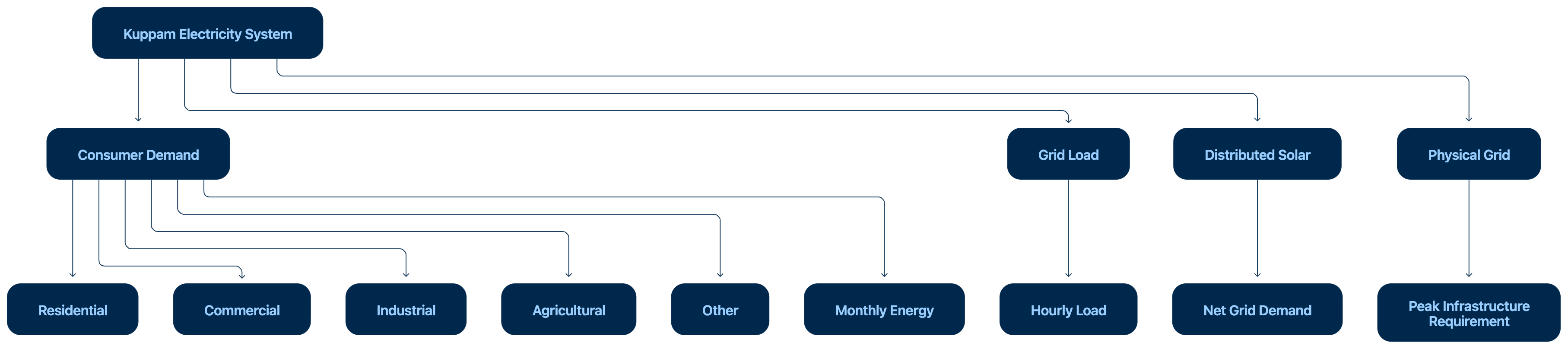 Figure 1: Regional Dataset Breakdown across 5 Mandals and 10 Consumer Categories
These datasets were all about electricity, but they were not measuring the same thing.
A consumer bill tells us how much energy was billed. Substation logs tell us instantaneous grid power draw. Solar generation offsets grid demand.
The system boundary comes before the model boundary.
Act II: Demand Disaggregation
3. One Region, Many Demand Processes
Aggregating all 10 consumer categories into a single historical series before forecasting would erase the mechanisms that actually generate demand.
Residential demand changes with population and appliance adoption. Commercial demand responds to economic activity. Agricultural demand is strongly tied to irrigation and cropping cycles.
Instead of forecasting one number, we forecast each consumer category separately and then aggregated the forecasts.
Act III: Organic vs Inorganic Growth Modeling
4. Organic vs. Inorganic Growth Vectors
Historical data is useful for learning organic demand growth. It is much less useful for predicting things that have never happened before (e.g. a future industrial park or EV charging plaza).
E_total(t) = ∑ E_organic,c(t) + E_inorganic(t)
We separated the forecast into two components:
- Organic demand: Population growth, historical consumption dynamics, weather, agricultural cycles.
- Inorganic demand: Planned industrial development, EV charging plazas, policy-driven agricultural solarization.
5. Forecasting the Part That History Could Explain
For the organic component, we used STL decomposition to separate long-term trend from short-term behavior, selected autoregressive lags using PACF, and trained a Random Forest model on the detrended series alongside climate variables (temperature, rainfall, sunshine hours, rainfall-regime indicators).
6. Turning Monthly Energy Into Hourly Load Profiles
Infrastructure does not fail because annual energy consumption is slightly higher than expected. It fails when instantaneous demand exceeds network capacity.
We used historical hourly grid-load data to construct representative 24-hour daily shapes (weekday, weekend, peak day, valley day) for each month.
We then scaled those historical hourly shapes by the future monthly energy predictions:
- Scaling Factor =
(Forecast Monthly Energy) / (Historical Monthly Energy) - Future Hourly Load =
(Historical Hourly Profile) × (Scaling Factor)
Act IV: System Architectural Insights
7. Changed Belief
Operator Takeaway
Initial belief: Regional energy forecasting is a time-series modeling problem.
Changed belief: Regional infrastructure forecasting is a system-modeling problem that happens to contain a time-series forecasting problem. Data architecture precedes model architecture.